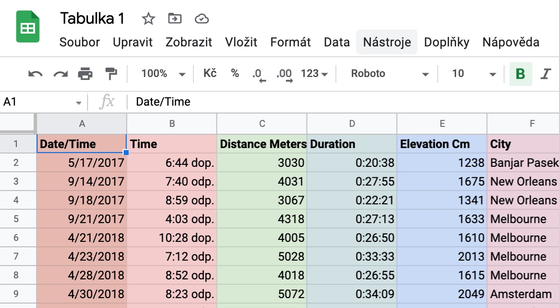
We continue our series on Google's online tools with a piece dedicated to the online spreadsheet processor Google Sheets. We will introduce you to five tips and tricks that will definitely come in handy when working with this web service.
It could be interest you

Cooperation
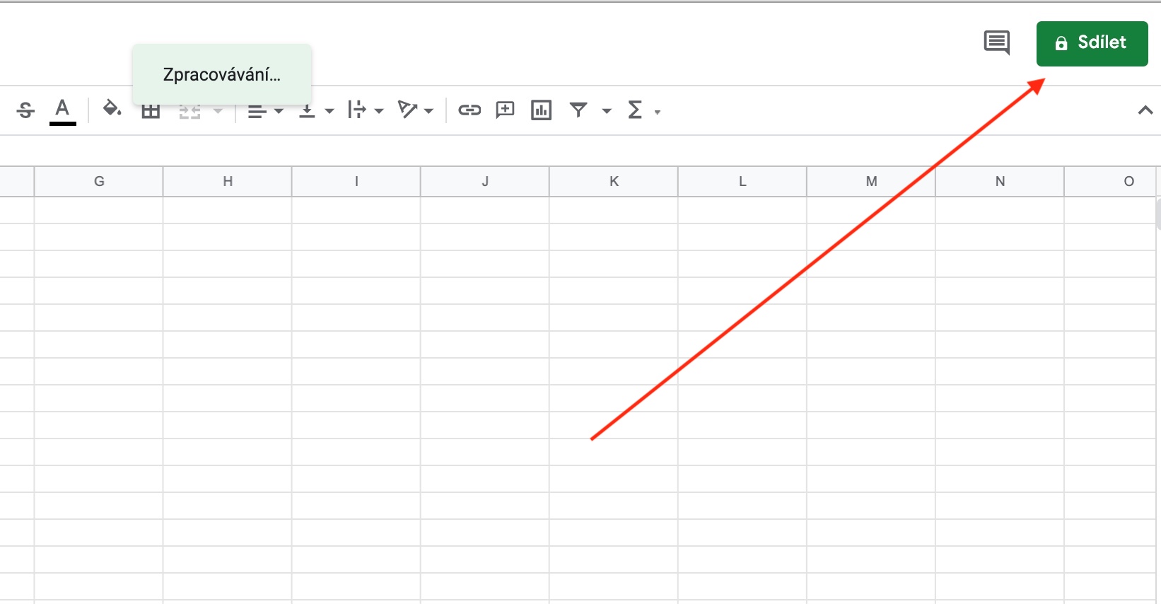
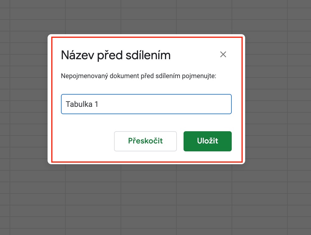
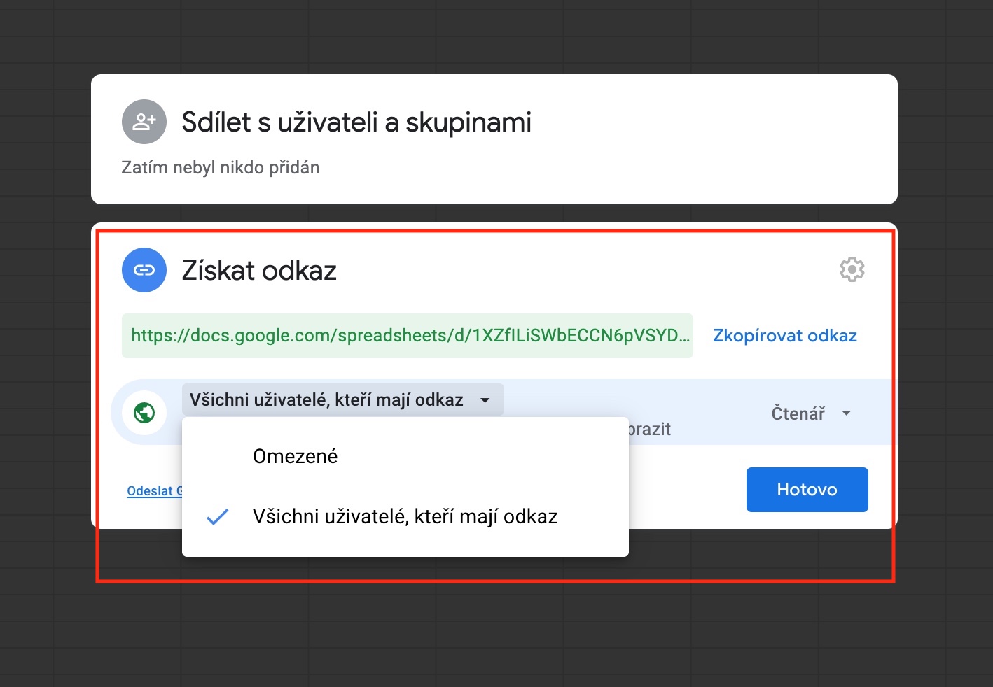
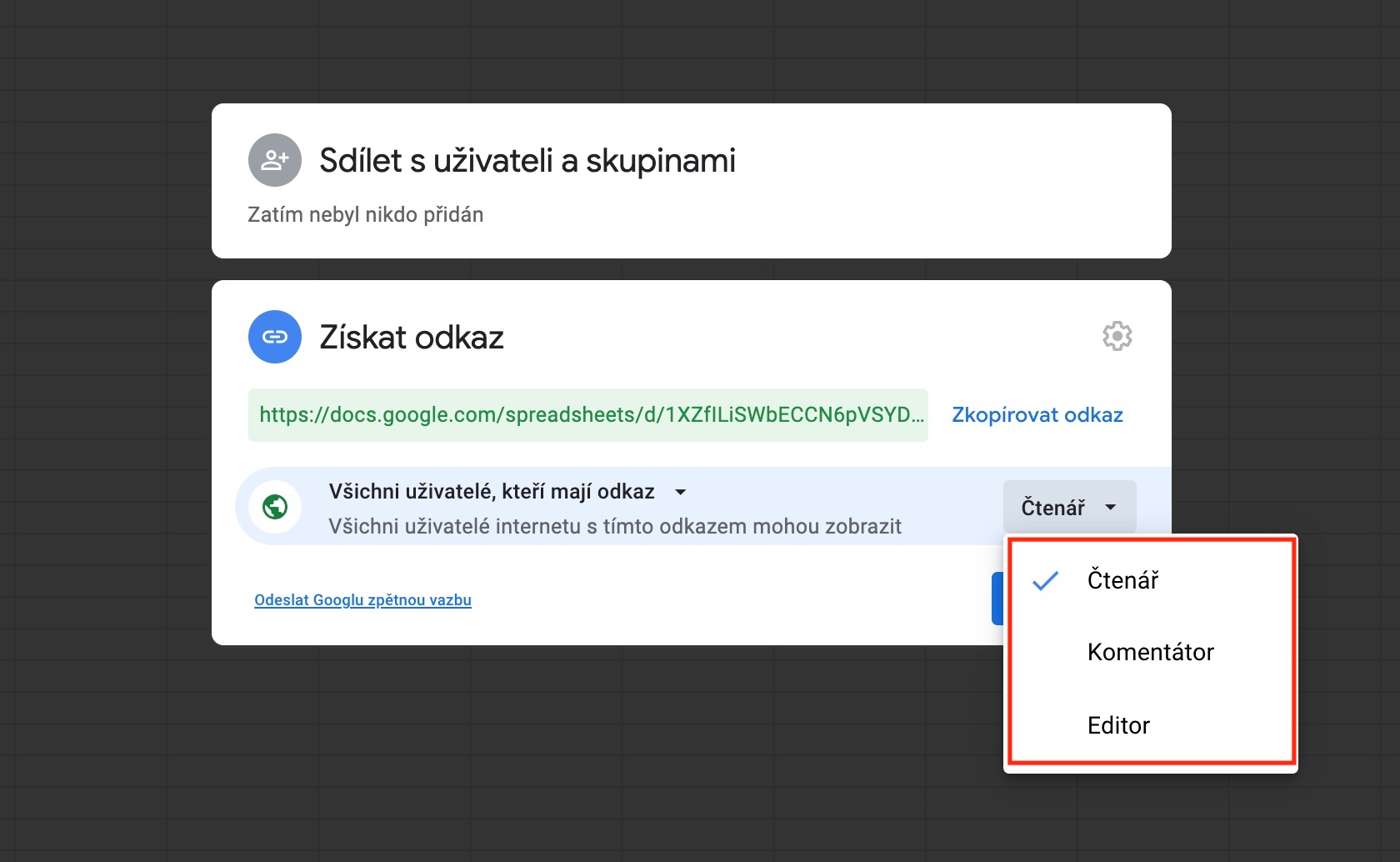
As with all other online services, you can also use the sharing and collaboration function in the case of Google Sheets - just click on in the upper right corner of the window with the table Share. Name the table and then v sharing tab click on "All users who have a link". You can then set sharing methods and permissions for those you share the table with.
Chart for better clarity
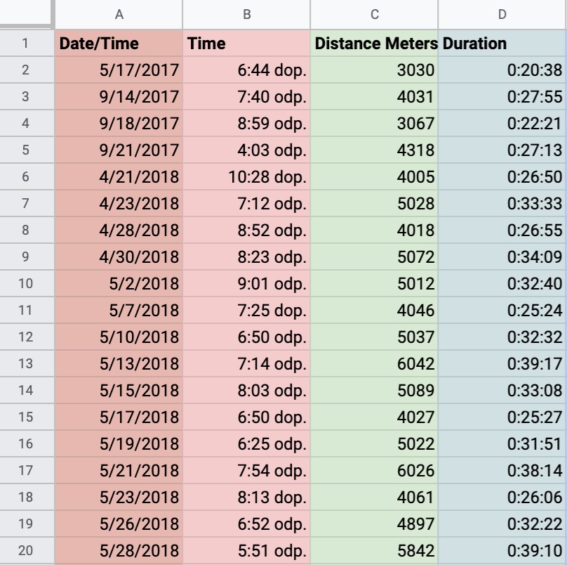
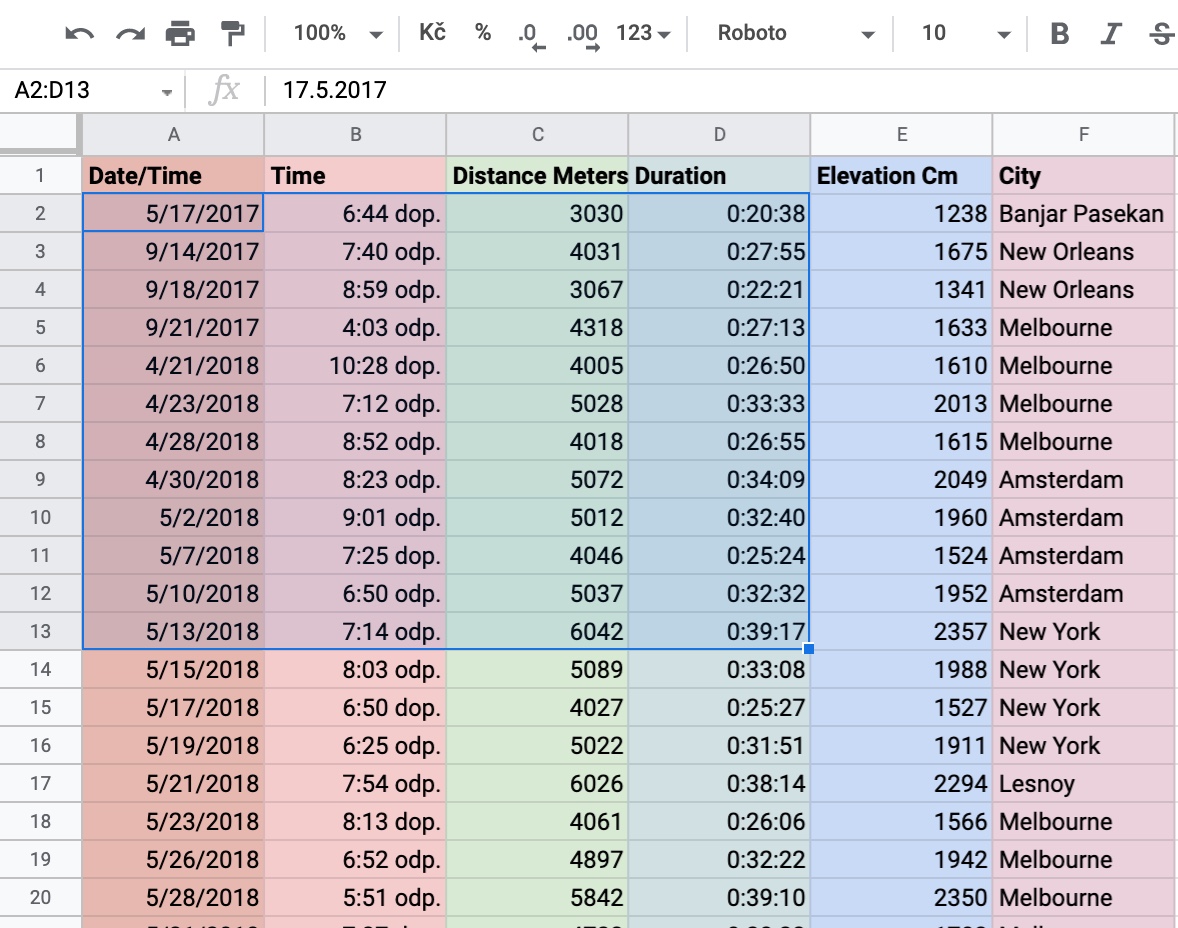
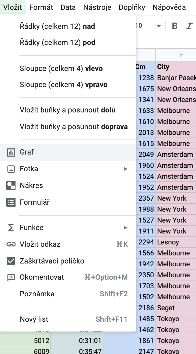
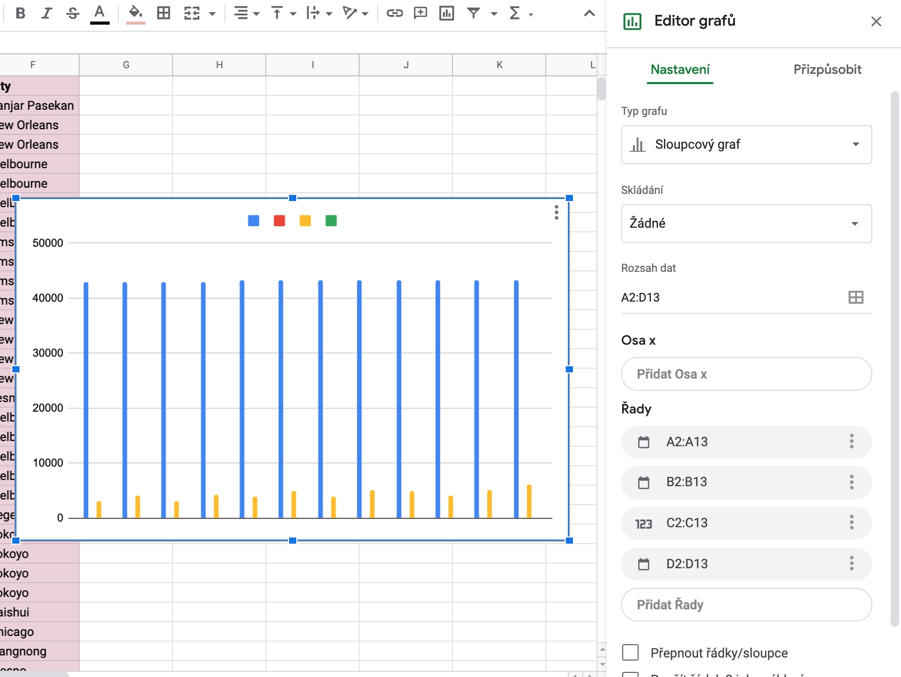
Tables in Google Sheets do not have to display the data you need in a classic way. If you want to make your table special or present the data in a different form, you can convert it into a color chart. The procedure is simple - just click in the table while holding down the Cmd key mark dates, which you want to convert to a graph, and then to toolbar at the top of the window Click on Insert -> Chart.
Cell locking
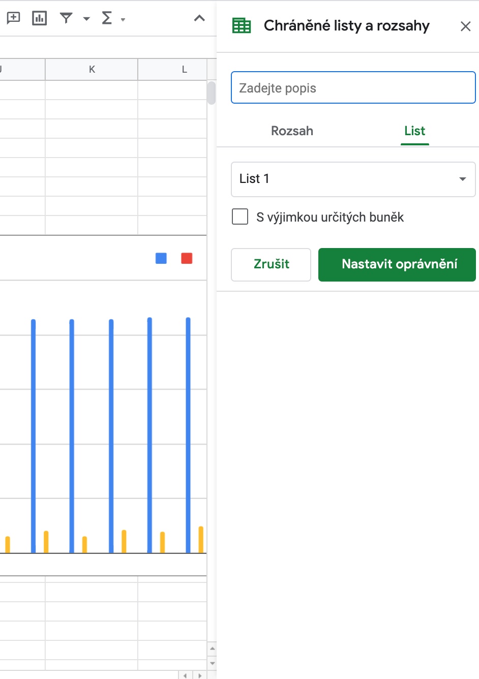
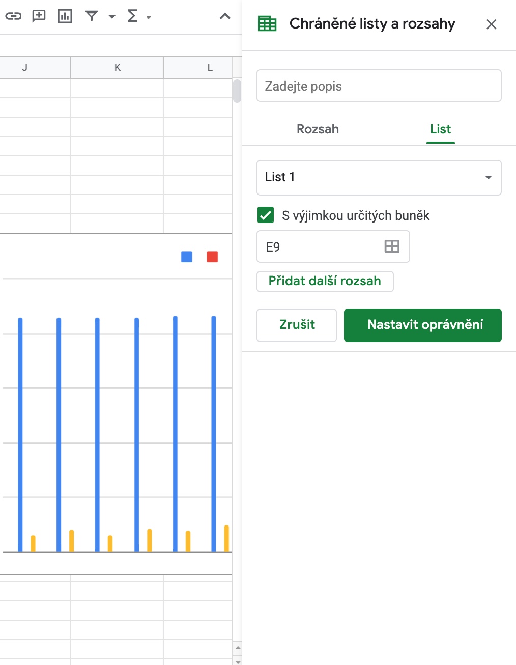
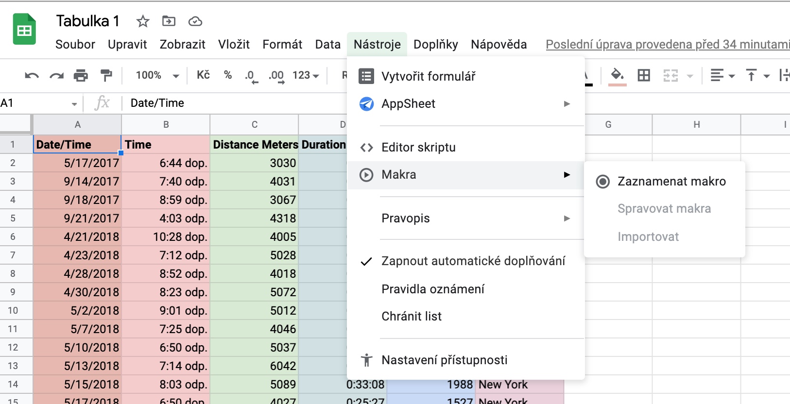
If you also share your spreadsheet with other users, and you don't want them to interfere with the selected cells in any way (which can also happen completely by accident and unintentionally), you can lock the data. You can lock both individual cells and the sheet as such. On toolbar at the top of the window click on Tools -> Protect sheet. After that in window set the locking parameters, or exclude the cells that you do not want to protect.
Macros
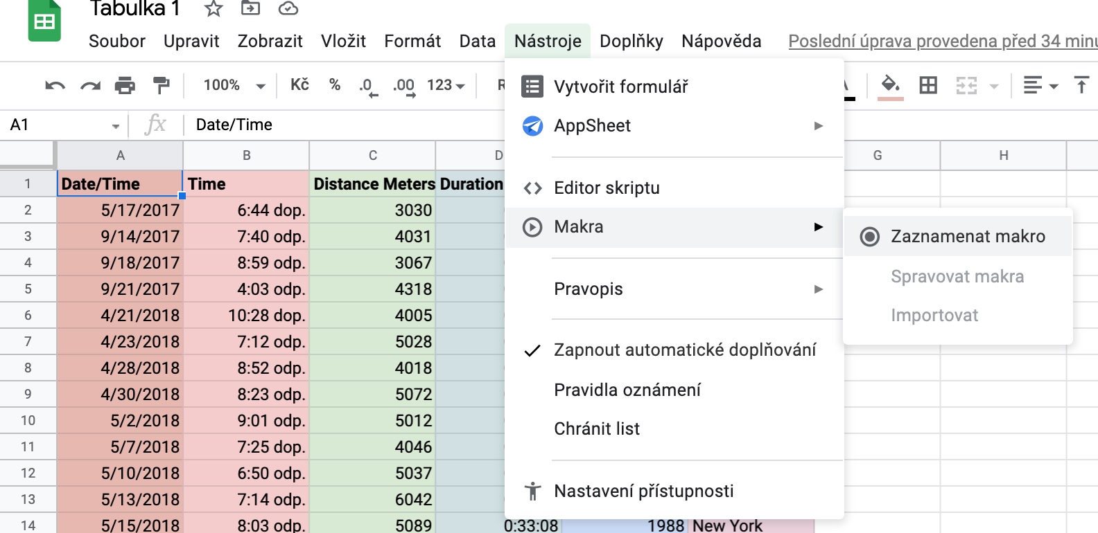
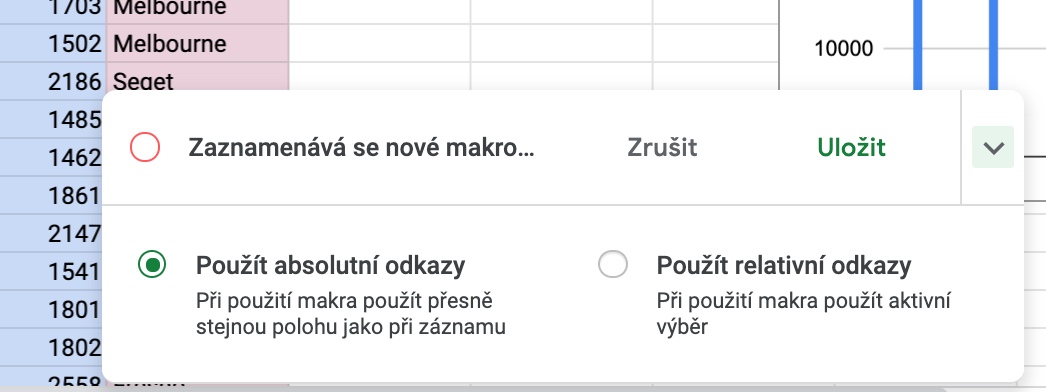
If you have been working with tables for a long time and in more detail, you are certainly familiar with the macro function from, for example, Microsoft Excel. However, you can also work with macros in the tables of the Google Sheets web application. On toolbar at the top of the window click on Tools -> Macros -> Record Macro. And lower part of the window will be displayed to you karta, where you set all the parameters and you can start recording.
